Imagine that an automobile manufacturer has developed prototypes for a new vehicle. Before introducing the new model into its range, the manufacturer wants to determine which existing vehicles on the market are most like the prototypes, i.e. how vehicles can be grouped, which group is the most similar with the model, and therefore which models they will be competing against.
In this blog post, we will use the heirarchical clustering to find the most distinctive clusters of vehicles. It will summarize the existing vehicles and help manufacturers to make a decision about the supply of new models.
# import libraries
import numpy as np
import pandas as pd
from matplotlib import pyplot as plt
from sklearn.cluster import AgglomerativeClustering
%matplotlib inline
# read the data into a pandas dataframe
filename = 'cars_clus.csv'
df = pd.read_csv(filename)

print('Shape of the dataframe: ', df.shape)
df.head()
Shape of the dataframe: (159, 16)
| manufact | model | sales | resale | type | price | engine_s | horsepow | wheelbas | width | length | curb_wgt | fuel_cap | mpg | lnsales | partition | |
|---|---|---|---|---|---|---|---|---|---|---|---|---|---|---|---|---|
| 0 | Acura | Integra | 16.919 | 16.360 | 0.000 | 21.500 | 1.800 | 140.000 | 101.200 | 67.300 | 172.400 | 2.639 | 13.200 | 28.000 | 2.828 | 0.0 |
| 1 | Acura | TL | 39.384 | 19.875 | 0.000 | 28.400 | 3.200 | 225.000 | 108.100 | 70.300 | 192.900 | 3.517 | 17.200 | 25.000 | 3.673 | 0.0 |
| 2 | Acura | CL | 14.114 | 18.225 | 0.000 | $null$ | 3.200 | 225.000 | 106.900 | 70.600 | 192.000 | 3.470 | 17.200 | 26.000 | 2.647 | 0.0 |
| 3 | Acura | RL | 8.588 | 29.725 | 0.000 | 42.000 | 3.500 | 210.000 | 114.600 | 71.400 | 196.600 | 3.850 | 18.000 | 22.000 | 2.150 | 0.0 |
| 4 | Audi | A4 | 20.397 | 22.255 | 0.000 | 23.990 | 1.800 | 150.000 | 102.600 | 68.200 | 178.000 | 2.998 | 16.400 | 27.000 | 3.015 | 0.0 |
The feature sets include price in thousands (price), engine size (engine_s), horsepower (horsepow), wheelbase (wheelbas), width (width), length (length), curb weight (curb_wgt), fuel capacity (fuel_cap) and fuel efficiency (mpg).
Data cleaning
Drop all the rows that have a null value.
print ("Size of dataset before cleaning: ", df.size)
df[[ 'sales', 'resale', 'type', 'price', 'engine_s',
       'horsepow', 'wheelbas', 'width', 'length', 'curb_wgt', 'fuel_cap',
       'mpg', 'lnsales']] = df[['sales', 'resale', 'type', 'price', 'engine_s',
       'horsepow', 'wheelbas', 'width', 'length', 'curb_wgt', 'fuel_cap',
       'mpg', 'lnsales']].apply(pd.to_numeric, errors='coerce')
df = df.dropna()
df = df.reset_index(drop=True)
print ("Size of dataset after cleaning: ", df.size)
df.head(5)
Size of dataset before cleaning:  2544
Size of dataset after cleaning:  1872
| manufact | model | sales | resale | type | price | engine_s | horsepow | wheelbas | width | length | curb_wgt | fuel_cap | mpg | lnsales | partition | |
|---|---|---|---|---|---|---|---|---|---|---|---|---|---|---|---|---|
| 0 | Acura | Integra | 16.919 | 16.360 | 0.0 | 21.50 | 1.8 | 140.0 | 101.2 | 67.3 | 172.4 | 2.639 | 13.2 | 28.0 | 2.828 | 0.0 |
| 1 | Acura | TL | 39.384 | 19.875 | 0.0 | 28.40 | 3.2 | 225.0 | 108.1 | 70.3 | 192.9 | 3.517 | 17.2 | 25.0 | 3.673 | 0.0 |
| 2 | Acura | RL | 8.588 | 29.725 | 0.0 | 42.00 | 3.5 | 210.0 | 114.6 | 71.4 | 196.6 | 3.850 | 18.0 | 22.0 | 2.150 | 0.0 |
| 3 | Audi | A4 | 20.397 | 22.255 | 0.0 | 23.99 | 1.8 | 150.0 | 102.6 | 68.2 | 178.0 | 2.998 | 16.4 | 27.0 | 3.015 | 0.0 |
| 4 | Audi | A6 | 18.780 | 23.555 | 0.0 | 33.95 | 2.8 | 200.0 | 108.7 | 76.1 | 192.0 | 3.561 | 18.5 | 22.0 | 2.933 | 0.0 |
Let’s select our feature set.
featureset = df[['engine_s', 'horsepow', 'wheelbas', 'width', 'length', 'curb_wgt', 'fuel_cap', 'mpg']]
Normalize the feature set.MinMaxScalar transforms features by scaling each feature to a given range. It is by default (0, 1). That is, the estimator scales and translates each feature individually such that is is betweeen 0 and 1.
from sklearn.preprocessing import MinMaxScaler
x = featureset.values #returns a numpy array
min_max_scaler = MinMaxScaler()
feature_mtx = min_max_scaler.fit_transform(x)
feature_mtx [0:5]
array([[0.11428571, 0.21518987, 0.18655098, 0.28143713, 0.30625832,
        0.2310559 , 0.13364055, 0.43333333],
       [0.31428571, 0.43037975, 0.3362256 , 0.46107784, 0.5792277 ,
        0.50372671, 0.31797235, 0.33333333],
       [0.35714286, 0.39240506, 0.47722343, 0.52694611, 0.62849534,
        0.60714286, 0.35483871, 0.23333333],
       [0.11428571, 0.24050633, 0.21691974, 0.33532934, 0.38082557,
        0.34254658, 0.28110599, 0.4       ],
       [0.25714286, 0.36708861, 0.34924078, 0.80838323, 0.56724368,
        0.5173913 , 0.37788018, 0.23333333]])
Clustering using Scipy
First, calculate the distance matrix.
import scipy
leng = feature_mtx.shape[0]
D = scipy.zeros([leng, leng])
for i in range(leng):
    for j in range(leng):
        D[i,j] = scipy.spatial.distance.euclidean(feature_mtx[i], feature_mtx[j])
C:\Users\prana\Anaconda3\lib\site-packages\ipykernel_launcher.py:3: DeprecationWarning: scipy.zeros is deprecated and will be removed in SciPy 2.0.0, use numpy.zeros instead
  This is separate from the ipykernel package so we can avoid doing imports until
In agglomerative clustering, at each iteration, the algorithm must update the distance matrix to reflect the distance of the newly formed cluster with the remaining clusters in the forest.
import pylab
import scipy.cluster.hierarchy
Z = hierarchy.linkage(D, 'complete')
C:\Users\prana\Anaconda3\lib\site-packages\ipykernel_launcher.py:3: ClusterWarning: scipy.cluster: The symmetric non-negative hollow observation matrix looks suspiciously like an uncondensed distance matrix
  This is separate from the ipykernel package so we can avoid doing imports until
Essentially, hierarchical clustering does not require a pre-specified number of clusters. However, in some application we might want a partition of disjoint clusters just as in flat clustering. So we can use a cutting line.
from scipy.cluster.hierarchy import fcluster
max_d = 3
clusters = fcluster(Z, max_d, criterion='distance')
clusters
array([ 1,  5,  5,  6,  5,  4,  6,  5,  5,  5,  5,  5,  4,  4,  5,  1,  6,
        5,  5,  5,  4,  2, 11,  6,  6,  5,  6,  5,  1,  6,  6, 10,  9,  8,
        9,  3,  5,  1,  7,  6,  5,  3,  5,  3,  8,  7,  9,  2,  6,  6,  5,
        4,  2,  1,  6,  5,  2,  7,  5,  5,  5,  4,  4,  3,  2,  6,  6,  5,
        7,  4,  7,  6,  6,  5,  3,  5,  5,  6,  5,  4,  4,  1,  6,  5,  5,
        5,  6,  4,  5,  4,  1,  6,  5,  6,  6,  5,  5,  5,  7,  7,  7,  2,
        2,  1,  2,  6,  5,  1,  1,  1,  7,  8,  1,  1,  6,  1,  1],
      dtype=int32)
You can determine the number of clusters directly.
from scipy.cluster.hierarchy import fcluster
k = 5
clusters = fcluster(Z,k, criterion='maxclust')
clusters
array([1, 3, 3, 3, 3, 2, 3, 3, 3, 3, 3, 3, 2, 2, 3, 1, 3, 3, 3, 3, 2, 1,
       5, 3, 3, 3, 3, 3, 1, 3, 3, 4, 4, 4, 4, 2, 3, 1, 3, 3, 3, 2, 3, 2,
       4, 3, 4, 1, 3, 3, 3, 2, 1, 1, 3, 3, 1, 3, 3, 3, 3, 2, 2, 2, 1, 3,
       3, 3, 3, 2, 3, 3, 3, 3, 2, 3, 3, 3, 3, 2, 2, 1, 3, 3, 3, 3, 3, 2,
       3, 2, 1, 3, 3, 3, 3, 3, 3, 3, 3, 3, 3, 1, 1, 1, 1, 3, 3, 1, 1, 1,
       3, 4, 1, 1, 3, 1, 1], dtype=int32)
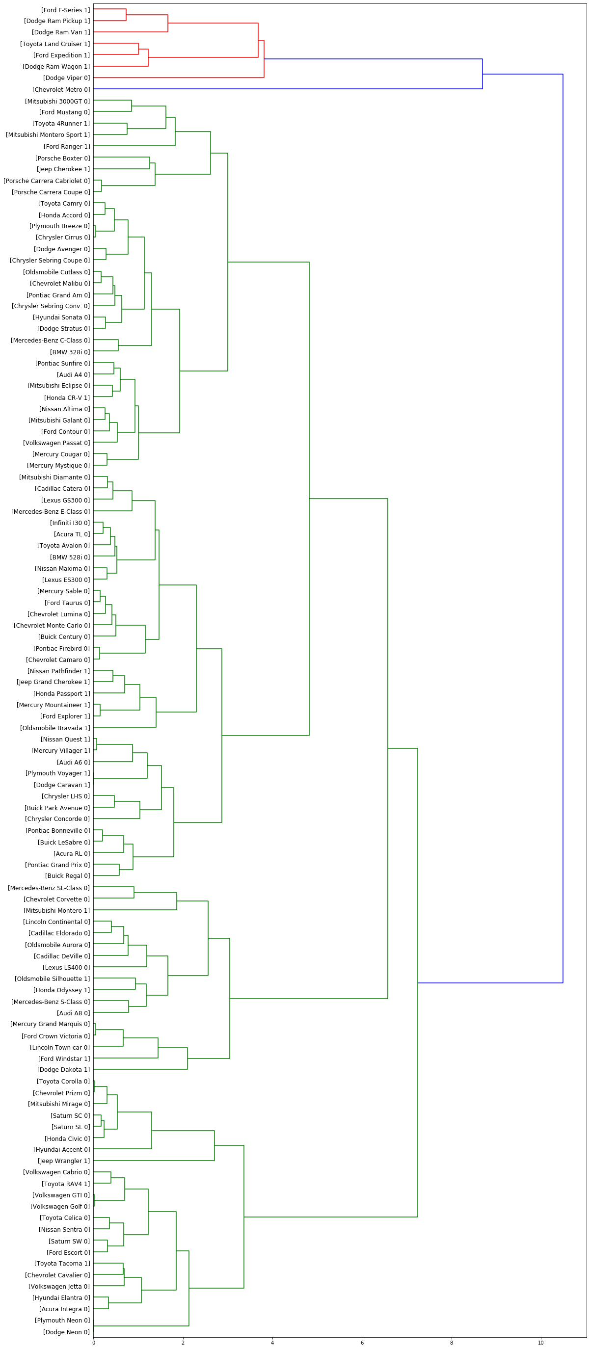
Plot the dendrogram.
fig = pylab.figure(figsize=(18,50))
def llf(id):
    return '[%s %s %s]' % (df['manufact'][id], df['model'][id], int(float(df['type'][id])) )

dendro = hierarchy.dendrogram(Z,  leaf_label_func=llf, leaf_rotation=0, leaf_font_size =12, orientation = 'right')
Clustering using scikit-learn
Let’s redo the above process using scikit-learn this time.
dist_matrix = distance_matrix(feature_mtx, feature_mtx)
print(dist_matrix)
[[0.         0.57777143 0.75455727 ... 0.28530295 0.24917241 0.18879995]
 [0.57777143 0.         0.22798938 ... 0.36087756 0.66346677 0.62201282]
 [0.75455727 0.22798938 0.         ... 0.51727787 0.81786095 0.77930119]
 ...
 [0.28530295 0.36087756 0.51727787 ... 0.         0.41797928 0.35720492]
 [0.24917241 0.66346677 0.81786095 ... 0.41797928 0.         0.15212198]
 [0.18879995 0.62201282 0.77930119 ... 0.35720492 0.15212198 0.        ]]
agglom = AgglomerativeClustering(n_clusters=6, linkage='complete')
agglom.fit(feature_mtx)
agglom.labels_
array([1, 2, 2, 1, 2, 3, 1, 2, 2, 2, 2, 2, 3, 3, 2, 1, 1, 2, 2, 2, 5, 1,
       4, 1, 1, 2, 1, 2, 1, 1, 1, 5, 0, 0, 0, 3, 2, 1, 2, 1, 2, 3, 2, 3,
       0, 3, 0, 1, 1, 1, 2, 3, 1, 1, 1, 2, 1, 1, 2, 2, 2, 3, 3, 3, 1, 1,
       1, 2, 1, 2, 2, 1, 1, 2, 3, 2, 3, 1, 2, 3, 5, 1, 1, 2, 3, 2, 1, 3,
       2, 3, 1, 1, 2, 1, 1, 2, 2, 2, 1, 1, 1, 1, 1, 1, 1, 1, 2, 1, 1, 1,
       2, 0, 1, 1, 1, 1, 1], dtype=int64)
We can add a new field to our dataframe to show the cluster of each row.
df['cluster_'] = agglom.labels_
df.head()
| manufact | model | sales | resale | type | price | engine_s | horsepow | wheelbas | width | length | curb_wgt | fuel_cap | mpg | lnsales | partition | cluster_ | |
|---|---|---|---|---|---|---|---|---|---|---|---|---|---|---|---|---|---|
| 0 | Acura | Integra | 16.919 | 16.360 | 0.0 | 21.50 | 1.8 | 140.0 | 101.2 | 67.3 | 172.4 | 2.639 | 13.2 | 28.0 | 2.828 | 0.0 | 1 |
| 1 | Acura | TL | 39.384 | 19.875 | 0.0 | 28.40 | 3.2 | 225.0 | 108.1 | 70.3 | 192.9 | 3.517 | 17.2 | 25.0 | 3.673 | 0.0 | 2 |
| 2 | Acura | RL | 8.588 | 29.725 | 0.0 | 42.00 | 3.5 | 210.0 | 114.6 | 71.4 | 196.6 | 3.850 | 18.0 | 22.0 | 2.150 | 0.0 | 2 |
| 3 | Audi | A4 | 20.397 | 22.255 | 0.0 | 23.99 | 1.8 | 150.0 | 102.6 | 68.2 | 178.0 | 2.998 | 16.4 | 27.0 | 3.015 | 0.0 | 1 |
| 4 | Audi | A6 | 18.780 | 23.555 | 0.0 | 33.95 | 2.8 | 200.0 | 108.7 | 76.1 | 192.0 | 3.561 | 18.5 | 22.0 | 2.933 | 0.0 | 2 |
import matplotlib.cm as cm
n_clusters = max(agglom.labels_)+1
colors = cm.rainbow(np.linspace(0, 1, n_clusters))
cluster_labels = list(range(0, n_clusters))

plt.figure(figsize=(12,10))

for color, label in zip(colors, cluster_labels):
    subset = df[df.cluster_ == label]
    for i in subset.index:
            plt.text(subset.horsepow[i], subset.mpg[i],str(subset['model'][i]), rotation=25)
    plt.scatter(subset.horsepow, subset.mpg, s= subset.price*10, c=color, label='cluster'+str(label),alpha=0.5)

plt.legend()
plt.title('Clusters')
plt.xlabel('horsepow')
plt.ylabel('mpg')
'c' argument looks like a single numeric RGB or RGBA sequence, which should be avoided as value-mapping will have precedence in case its length matches with 'x' & 'y'.  Please use a 2-D array with a single row if you really want to specify the same RGB or RGBA value for all points.
'c' argument looks like a single numeric RGB or RGBA sequence, which should be avoided as value-mapping will have precedence in case its length matches with 'x' & 'y'.  Please use a 2-D array with a single row if you really want to specify the same RGB or RGBA value for all points.
'c' argument looks like a single numeric RGB or RGBA sequence, which should be avoided as value-mapping will have precedence in case its length matches with 'x' & 'y'.  Please use a 2-D array with a single row if you really want to specify the same RGB or RGBA value for all points.
'c' argument looks like a single numeric RGB or RGBA sequence, which should be avoided as value-mapping will have precedence in case its length matches with 'x' & 'y'.  Please use a 2-D array with a single row if you really want to specify the same RGB or RGBA value for all points.
'c' argument looks like a single numeric RGB or RGBA sequence, which should be avoided as value-mapping will have precedence in case its length matches with 'x' & 'y'.  Please use a 2-D array with a single row if you really want to specify the same RGB or RGBA value for all points.
'c' argument looks like a single numeric RGB or RGBA sequence, which should be avoided as value-mapping will have precedence in case its length matches with 'x' & 'y'.  Please use a 2-D array with a single row if you really want to specify the same RGB or RGBA value for all points.


Text(0, 0.5, 'mpg')
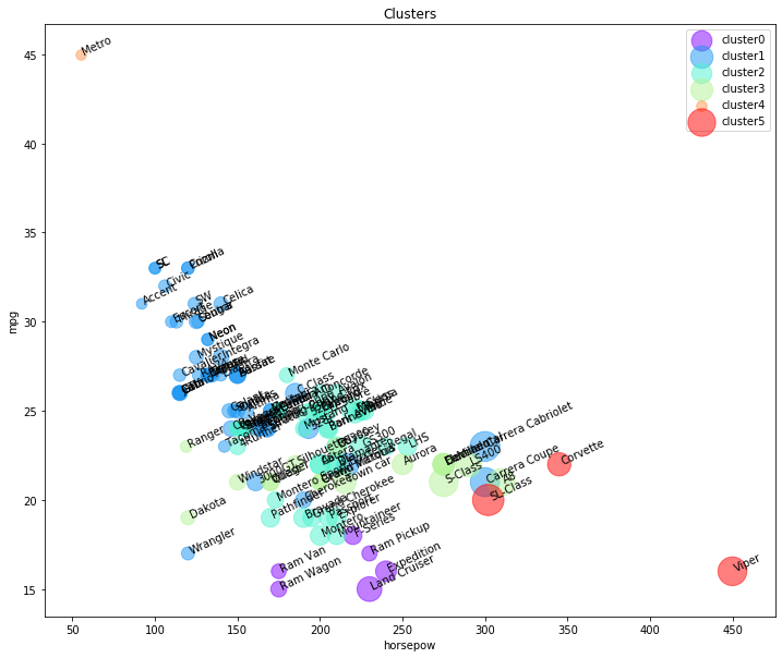
As you can see, we are seeing the distribution of each cluster using the scatter plot, but it is not very clear where is the centroid of each cluster. Moreover, there are 2 types of vehicles in our dataset, “truck” (value of 1 in the type column) and “car” (value of 0 in the type column). So, we use them to distinguish the classes, and summarize the cluster.
First we count the number of cases in each group.
df.groupby(['cluster_','type'])['cluster_'].count()
cluster_  type
0         1.0      6
1         0.0     47
          1.0      5
2         0.0     27
          1.0     11
3         0.0     10
          1.0      7
4         0.0      1
5         0.0      3
Name: cluster_, dtype: int64
Now we can look at the characteristics of each cluster.
agg_cars = df.groupby(['cluster_','type'])['horsepow','engine_s','mpg','price'].mean()
agg_cars
C:\Users\prana\Anaconda3\lib\site-packages\ipykernel_launcher.py:1: FutureWarning: Indexing with multiple keys (implicitly converted to a tuple of keys) will be deprecated, use a list instead.
  """Entry point for launching an IPython kernel.
| horsepow | engine_s | mpg | price | ||
|---|---|---|---|---|---|
| cluster_ | type | ||||
| 0 | 1.0 | 211.666667 | 4.483333 | 16.166667 | 29.024667 |
| 1 | 0.0 | 146.531915 | 2.246809 | 27.021277 | 20.306128 |
| 1.0 | 145.000000 | 2.580000 | 22.200000 | 17.009200 | |
| 2 | 0.0 | 203.111111 | 3.303704 | 24.214815 | 27.750593 |
| 1.0 | 182.090909 | 3.345455 | 20.181818 | 26.265364 | |
| 3 | 0.0 | 256.500000 | 4.410000 | 21.500000 | 42.870400 |
| 1.0 | 160.571429 | 3.071429 | 21.428571 | 21.527714 | |
| 4 | 0.0 | 55.000000 | 1.000000 | 45.000000 | 9.235000 |
| 5 | 0.0 | 365.666667 | 6.233333 | 19.333333 | 66.010000 |
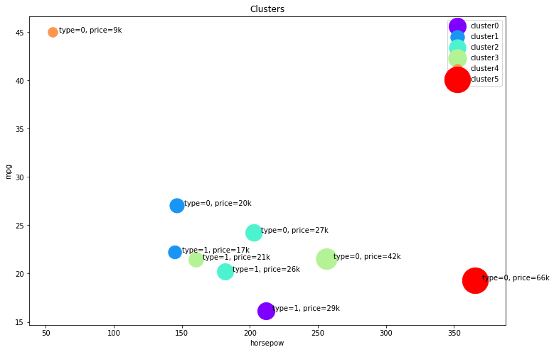
Cars:
- Cluster 1: low horsepower, high mileage, and low price
- Cluster 2: medium horsepower, medium mileage, and medium price
- Cluster 3: high horsepower, low mileage, and high price
- Cluster 4: very low horsepower, very high mileage, and very low price
- Cluster 5: very high horsepower, very low mileage, and very high price
Trucks:
- Cluster 0: high horsepower, low mileage, and high price
- Cluster 1: low horsepower, medium mileage, and low price
- Cluster 2: high horsepower, low mileage, and high price
- Cluster 3: low horsepower, low mileage, and medium price
plt.figure(figsize=(12,8))
for color, label in zip(colors, cluster_labels):
    subset = agg_cars.loc[(label,),]
    for i in subset.index:
        plt.text(subset.loc[i][0]+5, subset.loc[i][2], 'type='+str(int(i)) + ', price='+str(int(subset.loc[i][3]))+'k')
    plt.scatter(subset.horsepow, subset.mpg, s=subset.price*20, c=color, label='cluster'+str(label))
plt.legend()
plt.title('Clusters')
plt.xlabel('horsepow')
plt.ylabel('mpg')
'c' argument looks like a single numeric RGB or RGBA sequence, which should be avoided as value-mapping will have precedence in case its length matches with 'x' & 'y'.  Please use a 2-D array with a single row if you really want to specify the same RGB or RGBA value for all points.
'c' argument looks like a single numeric RGB or RGBA sequence, which should be avoided as value-mapping will have precedence in case its length matches with 'x' & 'y'.  Please use a 2-D array with a single row if you really want to specify the same RGB or RGBA value for all points.
'c' argument looks like a single numeric RGB or RGBA sequence, which should be avoided as value-mapping will have precedence in case its length matches with 'x' & 'y'.  Please use a 2-D array with a single row if you really want to specify the same RGB or RGBA value for all points.
'c' argument looks like a single numeric RGB or RGBA sequence, which should be avoided as value-mapping will have precedence in case its length matches with 'x' & 'y'.  Please use a 2-D array with a single row if you really want to specify the same RGB or RGBA value for all points.
'c' argument looks like a single numeric RGB or RGBA sequence, which should be avoided as value-mapping will have precedence in case its length matches with 'x' & 'y'.  Please use a 2-D array with a single row if you really want to specify the same RGB or RGBA value for all points.
'c' argument looks like a single numeric RGB or RGBA sequence, which should be avoided as value-mapping will have precedence in case its length matches with 'x' & 'y'.  Please use a 2-D array with a single row if you really want to specify the same RGB or RGBA value for all points.


Text(0, 0.5, 'mpg')